Bode plot of a simple pendulum

 

With a little assistance from ChatGPT, 

A Bode plot is a graphical representation of the frequency response of a system, which shows how a system responds to input signals of different frequencies. To make a Bode plot of a pendulum, you first need to model the pendulum mathematically as a system that responds to input signals.

Assuming that the pendulum is a simple pendulum, you can model it as a second-order system with a transfer function of the form:

G(s) = K / (s^2 + 2ζωn s + ωn^2)

where K is the gain, ωn is the natural frequency of the pendulum, and ζ is the damping ratio.

To obtain the Bode plot, you can plot the magnitude and phase of the transfer function G(s) as a function of frequency, ranging from 0 to infinity. To do this, you can express the transfer function in terms of frequency by substituting s = jω, where j is the imaginary unit and ω is the frequency in radians per second.

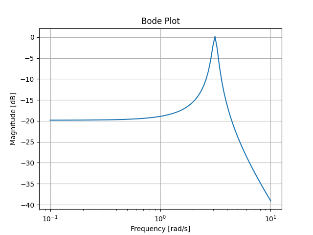
Once you have obtained the transfer function in terms of frequency, you can plot the magnitude and phase of G(jω) as a function of log(ω). The magnitude plot shows how the amplitude of the pendulum's response varies with frequency, while the phase plot shows how the phase of the response varies with frequency.

The Bode plot of a pendulum can provide insights into the system's stability and performance, and can be useful in designing control systems to regulate the pendulum's motion.

python code that will compute the transfer function of a pendulum of a given length and mass. and displays a bode plot

import numpy as np
from scipy import signal
from control import matlab
import matplotlib.pyplot as plt 

# Define pendulum parameters
l = 1.0   # length of pendulum in meters
m = 1.0   # mass of pendulum in kilograms
g = 9.81  # acceleration due to gravity in m/s^2 

# Compute natural frequency and damping ratio
wn = np.sqrt(g / l)
zeta = 0.05 

# Define transfer function
num = [1.0]
den = [1.0, 2*zeta*wn, wn**2]
G = signal.TransferFunction(num, den) 

# Compute frequency response
w, mag, phase = signal.bode(G)

# Compute frequency response
# omega = np.logspace(-2, 2, 1000)
# mag, phase, omega = matlab.bode(G, omega) 

# Display Bode plot
plt.figure()
plt.semilogx(w , mag)
plt.xlabel('Frequency [rad/s]')
plt.ylabel('Magnitude [dB]')
plt.title('Bode Plot')
plt.grid()
plt.show()

This code defines the length and mass of the pendulum, computes the natural frequency and damping ratio, and defines the transfer function using the signal.TransferFunction function. It then computes the frequency response using the matlab.bode function and displays the Bode plot using the matplotlib library. You can adjust the values of l, m, and zeta to see how they affect the Bode plot.